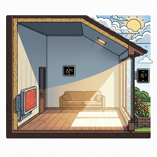
Imagine you're tasked with controlling the temperature in a smart home. You have a good model of the house's thermodynamics, you know how the heater works, and you measure both inside and outside temperature. But there's a catch: the sun. The amount of heat the house gains from the sun shining through the windows can be a huge, and unpredictable, factor. This is a classic example of a disturbance, an unknown input that affects our system.

In this blog post, we'll explore how to use Scientific Machine Learning (SciML) to learn a model of such a disturbance. We'll combine a physics-based model of a house's temperature with a small, interpretable neural network that learns the pattern of solar heat gain from data.

Failing to account for disturbances can have a deteriorating effect on many estimation and control tasks, for example

• If a disturbance is affecting a sensor, i.e., the sun is shining directly onto a thermometer, we must account for it in order to avoid biasing our state estimate. Failing to account for this may lead the control system to erroneously believe that the room is warmer than it actually is, resulting in inadequate heating.

• If a disturbance is affecting the system dynamics, we want to learn about it in order to let the controller compensate for it. In the case of our smart home, the sun heating the room must be met with a reduction in heater power to not make the room uncomfortably hot.

• When estimating model parameters, failing to account for disturbances can lead to biased parameter estimates and poor subsequent model performance, the optimizer will naturally use the optimized parameters to try to fit the disturbance if it has no other choice.

The System: A Simple Thermal Model

Let's start with what we know: the physics of our house. We can model the temperature of a single room using a simple differential equation based on Newton's law of cooling:

$$
\begin{align}
C_{thermal} \dot{T}(t) = -k_{loss} \big(T(t) - T_{ext}(t)\big) + \eta P_{heater}(t) + A_{window} I_{solar}(t)
\end{align}
$$

where:

• \(C_{thermal}\): thermal capacity of the room

• \(k_{loss}\): heat loss coefficient

• \(\eta\): heater efficiency

• \(A_{window}\): effective window area

• \(I_{solar}\): solar insolation (W/m²)

  
  

In plain English, this says that the rate of change of the room temperature \(T\) depends on:

• The heat loss to the outside, which is proportional to the temperature difference between the room \(T\) and the outside \(T_{ext}\).

• The power supplied by the heater \(P_{heater}\).

• The solar energy coming through the windows \(I_{solar}\).

We can simulate this scenario and look at the result:

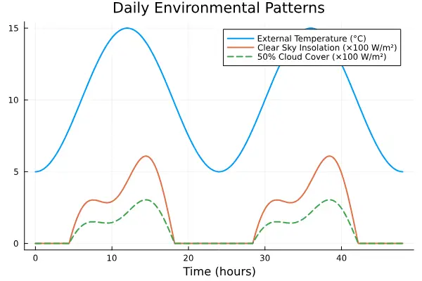
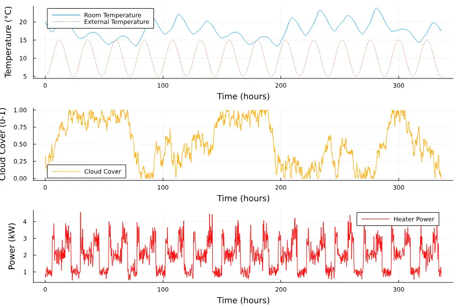
Here, we have two weeks of simulated data on which we will base our experiments. As you can see, the internal temperature increases during prolonged periods of low cloud cover.

Data-Driven Modeling of the Disturbance

Now for the tricky part: the solar insolation, \(I_{solar}\). This is our disturbance.

How the sun shines on a house on a cloud-free day, absent any surrounding trees or buildings, can be readily simulated. However, the real world offers a number of challenges that influence the effect this has on the inside temperature:

• Surrounding trees and buildings may cast shadows on the house at certain parts of the day.

• The sun shining in through a window has much greater effect than if it is shining on a wall.

• Cloud cover modulates the effect of the sun. The cloud cover is an unknown and stochastic variable which can change rapidly.

• As a vendor of, e.g., HVAC equipment with an interesting control system, you may not want to model each individual site in detail, including the location and size of windows and surrounding shading elements. Even if these are static, they are here thus to be considered unknown for the purposes of modeling for control.

We can model this situation as a combination of some deterministic parts and some stochastic parts, some known in advance and some yet to be learned. The path of the sun across the sky is certainly predictable, with one daily and one yearly component. The surroundings, like trees and buildings, are for the most part static, but the influence these have on the insolation is unknown, and so is the exact location and orientation of windows on the house. The heat gain from the sun moving across the sky, shining in through windows and being blocked by trees, is thus a deterministic but unknown function of time. However, the cloud cover modulating the sun intensity is stochastic. We can thus model the resulting insolation by:

• Treating the current cloud cover as a stochastic variable \(C_{cloud} \in [0, 1]\) to be estimated continuously. We achieve this by including the cloud cover as a state variable in our system. Absent any additional knowledge of this variable, we may model it as constant (zero deterministic time derivative) plus random noise, resulting in a random-walk model. We may also opt to let it slowly drift to the long-term average cloud cover absent any informative data.

• Treating the insolation when there is _no cloud cover_ as a deterministic function of the time of day (we ignore the yearly component here for simplicity). This function will be modeled as a basis-function expansion (one-layer neural network) that will be learned from data.

• The effective insolation at any point in time is thus \(I_{solar} = (1 - C_{cloud}) I_{solar, clear}\), that is, the cloud-free insolation \(I_{solar, clear}\) is modulated by the current (unknown) cloud cover to produce the effective insolation \(I_{solar}\).

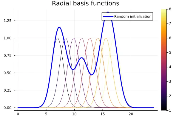
For the neural network, we don't need a huge, complex model. A simple Radial Basis Function (RBF) network will do the trick. An RBF network is just a weighted sum of Gaussian "bumps", which is a simple way of modeling a simple and smooth function of one variable.

# Initialize RBF weights (parameters to be learned)
rng = Random.default_rng()
Random.seed!(rng, 456)
const n_basis = 8  # Number of basis functions
# Initialize with positive weights since insolation is always positive ("negative insolation" could model things like someone always opening a window in the morning letting cold air in)
rbf_weights = 100.0f0 * rand(Float32, n_basis)  # Random positive initialization
function basis_functions(t)
    tod = time_of_day(t)
    centers = LinRange(7.0f0, 17.0f0, n_basis) # Centers spread from 07:00 to 17:00
    width = 1.5f0  # Width of each Gaussian basis function (in hours)
    @. exp(-((tod - centers) / width)^2)
end
# RBF evaluation function
function compute_nn_insolation(t, weights)
    return weights'basis_functions(t) # Linear combination of basis functions
end
ts = 0:0.1:24
plot(ts, reduce(hcat, basis_functions.(ts))', title="Radial basis functions", lab="", line_z=(1:n_basis)', palette = :inferno)
plot!(ts, compute_nn_insolation.(ts, Ref(rbf_weights)) ./ 100, lab="Random initialization", l=(3, :blue))

Enforcing Constraints with a Sigmoid Transformation

We'll use an Unscented Kalman Filter to estimate the room temperature and the cloud cover. But we have a constraint: the cloud cover is by definition a variable between 0 and 1. The Kalman filter framework doesn't natively handle such constraints, but we can work around this by a simple heuristic.

A neat trick to handle this is to estimate the cloud cover in a transformed space. We can use the inverse of the sigmoid function (also known as the logit function) to map the [0, 1] interval to the entire real line. Then, inside our dynamics model, we can use the sigmoid function to map the variable to the [0, 1] interval.

Here's how we can write our dynamics function using this trick:

sigmoid(x) = 1 / (1 + exp(-x))
sigmoid_inv(y) = log(y / (1 - y))
function thermal_dynamics_sigmoid(x, u, p, t)
    T_room, log_cloud_cover = x
    cloud_cover = sigmoid(log_cloud_cover)
    P_heater = u[1]
    # External temperature (known from an outside sensor)
    T_ext = external_temp(t)
    # Solar insolation from RBF model
    I_base = compute_nn_insolation(t, p)
    I_solar = I_base * (1 - cloud_cover)
    # Heat balance
    dT_dt = (-k_loss * (T_room - T_ext) + η * P_heater + A_window * I_solar / 1000) / C_thermal
    # Cloud cover changes slowly (in transformed space)
    dlogcloud_dt = 0.0001f0*(sigmoid_inv(0.5f0) - log_cloud_cover) # a random walk with a slow bias towards 50% cloud cover
    SA[dT_dt, dlogcloud_dt]
end

Putting it all Together

Now we have all the pieces:

• A physical model of the house.

• A neural network model the cloud-free solar insolation.

• A Kalman filter to estimate the room temperature and cloud cover.

• A way to handle the cloud cover constraint.

Parameter Estimation

To learn the insolation pattern over time, we'll set up the state estimator (UKF) and minimize the one-step prediction errors using a gradient-based quasi-Newton method. The technical details on how this optimization is performed are left out here for brevity, but are included in the accompanying notebook.

Results of Optimization Algorithm
 * Algorithm: LevenbergMarquardt
 * Minimizer: [359.7153,37.799362,286.70786,11.353377,505.9033,162.80666,542.91125,62.937122]
 * Sum of squares at Minimum: 21.893978
 * Iterations: 18
 * Convergence: true
 * |x - x'| < 1.0e-08: false
 * |f(x) - f(x')| / |f(x)| < 1.0e-08: true
 * |g(x)| <

The result is obtained very quickly (less than 0.1 seconds), a benefit of using a neural network no larger than required

timing.time # seconds

0.070704695

Let's analyze the results of the optimization by running the filter with optimized parameters:

# Run filter with optimized parameters and linear measurement model
kf_final = UnscentedKalmanFilter(
    discrete_dynamics_hybrid,
    measurement_model,
    R1,
    SimpleMvNormal(x0, R1);
    p = params_opt,
    ny, nu, Ts
)
sol = forward_trajectory(kf_final, data.u, data.y)
# Extract estimated state trajectories
T_est = [sol.xt[i][1] for i in 1:length(sol.xt)]
cloud_est = [sigmoid.(sol.xt[i][2]) for i in 1:length(sol.xt)]
T_true = [data.x[i][1] for i in 1:length(data.x)]
cloud_true = [data.x[i][2] for i in 1:length(data.x)]
# Only compute cloud RMSE when sun is above horizon
sun_up_mask = [true_insolation(data.t[i], 0.0f0) > 0 for i in 1:length(data.t)]
cloud_error = sqrt(mean(abs2, cloud_true[sun_up_mask] .- cloud_est[sun_up_mask]))
# Plot temperature estimation
p1 = plot(data.t, T_true, label="True Temperature", lw=2, color=:blue)
plot!(data.t, T_est, label="Estimated Temperature", lw=2, ls=:dash, color=:red)
plot!(data.t, [y[1] for y in data.y], label="Measurements", alpha=0.3, seriestype=:scatter, ms=1, color=:gray)
ylabel!("Temperature (°C)")
title!("Temperature Estimation")
# Plot cloud cover estimation
p2 = plot(data.t, cloud_true, label="True Cloud Cover", lw=2, color=:blue)
plot!(data.t, cloud_est, label="Estimated Cloud Cover", lw=2, ls=:dash, color=:red)
ylabel!("Cloud Cover")
xlabel!("Time (hours)")
title!("Cloud Cover Estimation")
add_background_shading!(p1, data.t, sun_up_mask)
add_background_shading!(p2, data.t, sun_up_mask)
plot(p1, p2, layout=(2,1), size=(1200, 800))

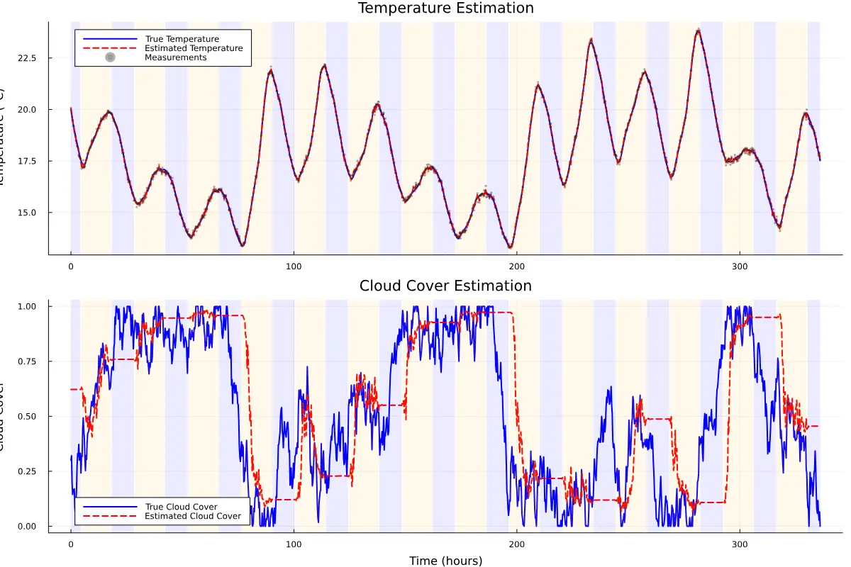
As we can see, it's easy to estimate the internal temperature, after all, we measure this directly. Estimating the cloud cover is significantly harder, during daytime we do a reasonable job but notice in particular how the estimate appears to get stuck each night when there is no sun. This is expected since under our assumed dynamical model, it is impossible to observe (in the estimation-theoretical sense) the cloud cover when there is no sun, when there is no sun there is no effect of the cloud cover on the variable we do measure, the temperature. Thankfully, having an estimate of the cloud cover during the day is all that it takes to learn about insolation patterns.

Learned vs True Insolation Pattern

We now have a look at the function we learned for the effect of insolation on the internal temperature, absent of clouds. Since this is a simulated example, we have access to the true function to compare with:

# Generate time points for one day
tod_test = LinRange(0.0f0, 24.0f0, 100)
# Compute true insolation (without clouds)
I_true = [true_insolation(t, 0.0f0) for t in tod_test]
# Compute learned insolation
I_learned = [compute_nn_insolation(t, params_opt) for t in tod_test]
# Plot comparison
plot(tod_test, I_true, label="True Insolation", lw=3, color=:blue)
plot!(tod_test, I_learned, label="Learned Insolation", lw=2, ls=:dash, color=:red)
xlabel!("Time of Day (hours)")
ylabel!("Insolation (W/m²)")
title!("Learned Solar Insolation Pattern")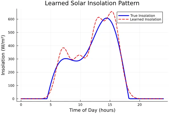

Hopefully, we see that the estimation has captured the general shape of the true insolation pattern, but perhaps not perfectly, since this function is "hidden" behind an unknown and noisy estimate of the cloud cover. In this example, we used 14 days worth of data, one would expect this estimate to improve the more data is used.

Discussion

This example demonstrates a classical SciML workflow, the combination of physics-based thermal dynamics with a data-driven model to capture unknown solar patterns. During the day, we were able to roughly estimate the cloud cover despite this not being directly measured, by leveraging its effect on the temperature dynamics. However, during night our estimator has no fighting chance of doing a good job here, a limitation inherent to the unobservability of the cloud cover in the absence of sunlight.

By learning a disturbance model like this, a smart control system can, e.g., proactively reduce heat input in rooms with significant insolation on forecasted sunny days. In a similar way, we could use this functionality to learn things like occupancy patterns and their impact on room temperature, and outside the example of temperature control, we can imagine applications like

• Environmental modeling: Weather, soil moisture, or unobserved interactions affect ecological or hydrological systems. For example, modeling of soil evaporation rates in agricultural water balance models.

• Aerospace: An aircraft’s flight dynamics are influenced by turbulent wind gusts that are difficult to model from first principles.

• Vehicle dynamics: Capturing driver-specific behavior in vehicle dynamics.