

Across mechanical, thermal, and controls engineering, a persistent workflow fragmentation exists between two fundamental analysis modes. Steady-state analysis determines the equilibrium operating point and equipment capacity requirements under design-load conditions. Transient analysis evaluates the system's dynamic response to time-varying inputs, disturbances, and off-design events, and control signals. Both are applied to the same physical plant — yet in practice, they operate on separate representations of the model maintained in separate tools.
When a parameter is updated in the sizing model, it must be manually propagated to the simulation model. Over successive design iterations, these representations diverge. The result is inconsistency between the equipment specifications derived from steady-state analysis and the operational behavior predicted by transient simulation.
This post demonstrates an alternative: a single acausal thermal model of a three-zone commercial office building in Dyad, which is run in steady state as well as transient modes. The steady state model computes sizing of the HVAC equipment, subject to fixed boundary conditions, and the transient analysis analyzes building performance over a 24-hour diurnal operation. The base model has identical parameters and governing equations in both cases.
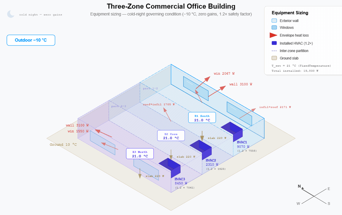
Figure 1: Three-Zone Commercial Office Building — isometric cutaway showing the thermal network, envelope heat flows, and HVAC units at design-day conditions
The rest of this post is designed as the following: first, we examine how this model fragmentation occurs across the CAE industry. Next, we will walk through an example of a three-zone commercial building and demonstrate how both equipment sizing and occupancy demand response analysis can be performed off a single source of truth in Dyad.
The Fragmentation Is Domain-Independent
The steady-state/transient split manifests across every major CAE discipline. The table below illustrates the pattern: the same physical plant requires both analysis modes, yet the parameters that govern both are maintained in separate versions of the same physical equipment — one for sizing, another for simulation. These models are often written and maintained in separate software packages. For example, propulsion modeling in aircraft relies on software like NPSS for design point thrust computation, but then moves to software like T-MATs for transient engine analysis during flight maneuvers.
Domain | Application for Steady State | Application for Transient |
HVAC/Buildings | Peak heating/cooling loads at design-day conditions; duct/pipe sizing; air handler selection; ASHRAE 90.1 code compliance; thermostat gain tuning; chiller plant sequencing | Diurnal zone temperature trajectories; cold-start warmup time; thermostat cycling; pre-cooling/pre-heating demand response strategies; sensor drift and stuck-valve fault detection |
Aerospace — Propulsion | Design-point thrust/SFC; compressor/turbine matching; off-design performance maps; avionics cooling and ECS sizing; heat exchanger rating; FADEC logic verification | Accel/decel fuel schedule response; compressor surge during rapid throttle; flame-out recovery; turbine blade soak-back after shutdown; bearing oil coking; ice crystal ingestion |
Aerospace — Airframe | Steady-level-flight load envelopes; structural weight estimation; fuel flow distribution and pump sizing at cruise; cabin pressure/temperature at cruise; bleed air pack capacity | Dynamic gust response; flutter onset; landing gear impact loads; fuel slosh during maneuvers; tank transfer transients; rapid cabin depressurization; emergency descent oxygen demand |
Automotive — Powertrain | Torque/power/BSFC maps; turbo matching; EGR sizing; gear ratio optimization; torque converter matching; battery thermal equilibrium at rated charge/discharge; coolant loop sizing | WLTP/FTP drive cycle fuel consumption; hybrid mode transitions; boost pressure transient during tip-in; wastegate dynamics; cell temperature rise during fast charge; thermal runaway propagation |
Chemical / Process | Heat & mass balance at rated throughput; reactor and column sizing; pipe network pressure drop; pump head requirements; relief valve sizing; heat exchanger UA rating and fouling allowance | Reactor temperature ramp during startup; distillation column flooding; catalyst activation; batch reaction profiles; endpoint detection; pressure vessel blowdown; runaway reaction progression |
Comparing these columns reveals a systematic pattern: in nearly every domain, the steady-state and transient problems are addressed by separate model representations — frequently maintained in different tools, with incompatible formats and separate parameter databases. The building thermal network is described once for peak load sizing and again for annual energy simulation. The gas turbine cycle is described once for design-point analysis and again for control system development. The chemical process is described once for heat and mass balance and again for startup/shutdown studies.
This approach leads to inconsistency between the models that develop over the course of the product lifecycle. Dyad helps eliminate this inconsistency by supporting multiple analysis types on a single model representation.
System Under Study: Three-Zone Commercial Office Building
The demonstration model represents a commercial office partitioned into three thermal zones: a south-facing perimeter zone (Z1), an interior core zone (Z2), and a north-facing perimeter zone (Z3). The thermal network comprises:
Envelope resistance elements — wall, window, roof, slab-on-grade, and infiltration thermal resistors per zone, parameterized by R-value (K/W)
Zone thermal capacitances — lumped-parameter heat capacitors (C in J/K) representing the aggregate thermal mass of each zone
Inter-zone conduction paths — thermal resistors coupling adjacent zones through interior partition walls
Boundary condition signal inputs — outdoor air and ground temperatures enter as causal RealInput signal ports, converted internally to thermal boundary conditions via PrescribedTemperature sources
External zone ports — each zone exposes a single thermal Node port for connecting any combination of HVAC equipment, internal gains, and solar loads. The building model is agnostic to the control law; heating/cooling sources are attached at the test-harness level.
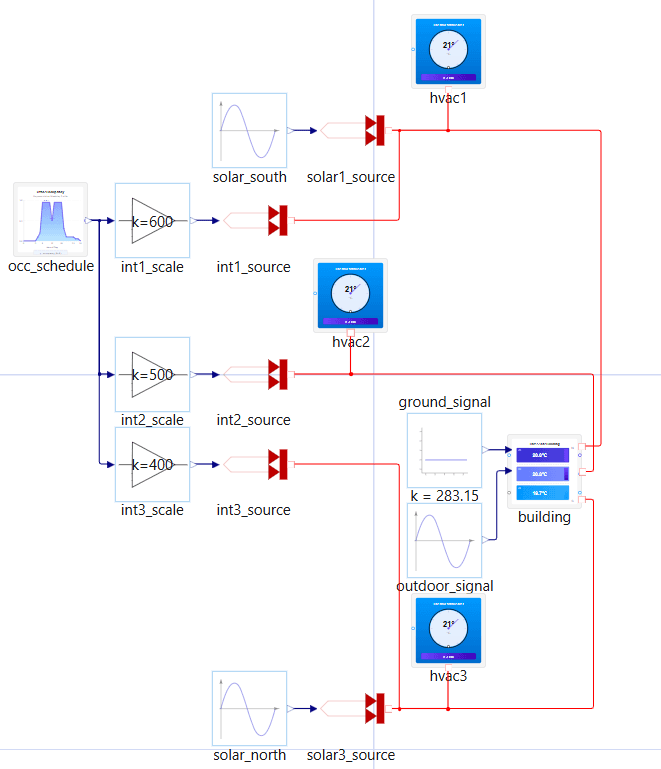
The model — `ThreeZoneBuilding` — exposes two causal signal inputs (outdoor temperature, ground temperature) and three thermal Node ports (one per zone for HVAC, gains, and external loads), encapsulating all internal physics. It is agnostic to the nature of the boundary conditions and HVAC strategy attached at these ports.
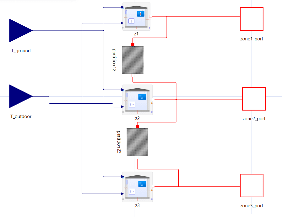
Figure 2: Schematic of Three Zone Commercial Building.
Three test harnesses supply boundary conditions to the same ThreeZoneBuilding instance:
TestSteadySizing — occupied design-day conditions (outdoor: −5°C, ground: 10°C) with fixed internal gains (600, 500, 400 W per zone) and design-average solar irradiance (1500 W south, 375 W north). FixedTemperature boundary conditions at 21°C are applied directly to each HVAC port, imposing the desired zone temperature as an algebraic constraint. The solver determines the heat flow Q through each port — this is the required HVAC capacity, obtained without any controller or equipment model.
TestColdNightSizing — unoccupied cold-night conditions (outdoor: −10°C, ground: 10°C) with zero internal and solar gains. Same FixedTemperature setpoints at 21°C. This captures the worst-case heating demand that occurs at the coldest hour with no solar or occupancy offset.
TestDiurnalOperation — sinusoidal outdoor temperature (−10°C to 0°C, 24-hour period), a representative weekday office occupancy schedule scaled to zone-specific internal gains, and sinusoidal solar gains with noon peak. Realistic proportional controllers (K = 5000 W/K) provide thermostat control, with installed capacities set to the governing sizing condition per zone.
All three test harnesses draw from the identical thermal network and parameter set. Only the boundary conditions and HVAC strategy differ.
Steady-State Analysis: Equilibrium Operating Point and Equipment Capacity
The SteadyStateAnalysis formulates the system as a coupled algebraic problem by setting dT/dt = 0 for all thermal capacitances. With FixedTemperature boundary conditions imposed at each HVAC port, the zone temperatures are algebraically determined — the solver computes the heat flow Q through each port required to maintain 21°C against the envelope losses. This is a direct equilibrium computation — not a time-integration run to convergence, and not a controller-based approximation.
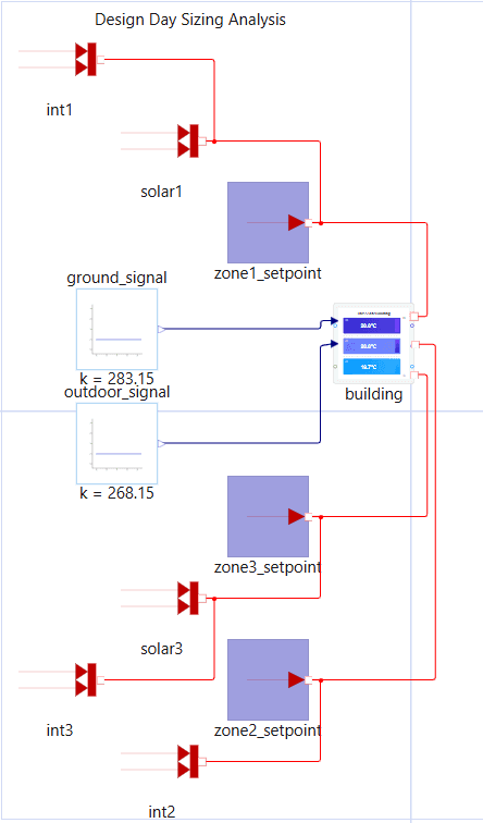
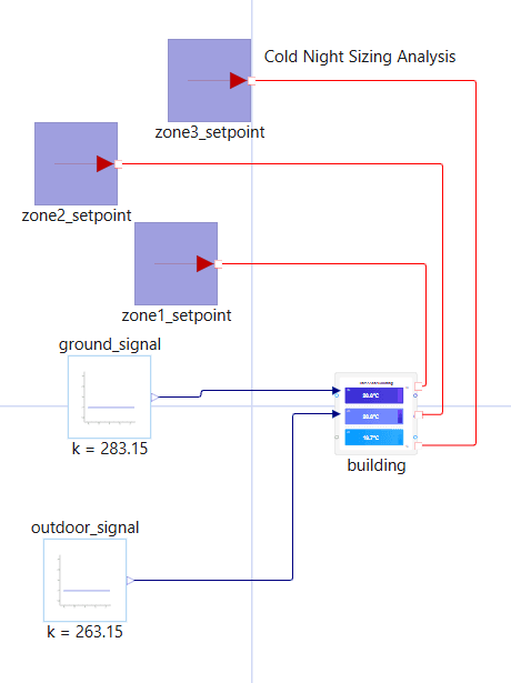
Figure 3: Two test harnesses imposing two sets of fixed boundary conditions, the first corresponding to design day conditions and the second corresponding to cold night conditions.
Condition 1 — Occupied design day (−5°C outdoor, with solar and internal gains):
Zone | Required HVAC Capacity | Envelope Loss | Internal + Solar Gains |
|---|---|---|---|
Z1 (South) | 4,274 W | 6,374 W | 600 + 1,500 W |
Z2 (Core) | 1,150 W | 1,650 W | 500 W |
Z3 (North) | 5,166 W | 5,941 W | 400 + 375 W |
Condition 2 — Unoccupied cold night (−10°C outdoor, zero gains):
Zone | Required HVAC Capacity | Envelope Loss | Internal + Solar Gains |
|---|---|---|---|
Z1 (South) | 7,558 W | 7,558 W | 0 W |
Z2 (Core) | 1,925 W | 1,925 W | 0 W |
Z3 (North) | 7,041 W | 7,041 W | 0 W |
Putting it together, the following capacities were finalized.
Zone | Required Capacity | With 1.2× Safety Factor |
|---|---|---|
Z1 (South) | 7,558 W | 9,070 W |
Z2 (Core) | 1,925 W | 2,310 W |
Z3 (North) | 7,041 W | 8,450 W |
Building Total | 16.5 kW | 19.8 kW |
This dual-condition approach reveals that a south-facing zone sized only for the occupied design day would be undersized for cold-night operation. At −5°C with 1,500 W of solar gain, Z1 requires only 4,274 W — but at −10°C with zero solar, the same zone requires 7,558 W. The 1,500 W solar credit that reduces the design-day load vanishes entirely at night, and the 5 K colder outdoor temperature increases envelope losses by 30%. Both conditions are evaluated on the identical thermal network, with only the boundary conditions differing between the two SteadyStateAnalysis invocations.
Transient Analysis: Dynamic Response Under Diurnal Boundary Conditions and Occupancy
The identical `ThreeZoneBuilding` — with the same governing equations and parameter values — is subjected to `TransientAnalysis` over an 86,400-second (24-hour) simulation horizon with time-varying boundary conditions. Realistic proportional thermostat controllers (K = 5000 W/K) are attached at the test-harness level, with installed capacities set to 1.2× the governing sizing result per zone: Q_max = 9,070 W (Z1), 2,310 W (Z2), and 8,450 W (Z3). There are two time-varying boundary boundary conditions imposed: a representative occupancy schedule, as well as sinusoidal solar sources that reach their peak at 12:00 hours.
Occupancy Model: Representative Weekday Office Profile
Internal gains in each zone are modulated by a time-varying occupancy fraction representing a typical weekday office usage pattern. The `OfficeOccupancy` component implements this as a piecewise-linear interpolation between hourly breakpoints, outputting a dimensionless fraction (0–1) that scales each zone's peak internal gain:
Hour | Fraction | Period |
|---|---|---|
0:00–5:00 | 0.00 | Unoccupied overnight |
5:00–6:00 | 0.00 → 0.10 | Early arrival ramp |
6:00–7:00 | 0.10 → 0.20 | Morning ramp-up |
7:00–8:00 | 0.20 → 0.95 | Staff arrival |
8:00–11:00 | 0.95 | Morning peak |
11:00–12:00 | 0.95 → 0.50 | Lunch departure |
12:00–13:00 | 0.50 → 0.95 | Lunch return |
13:00–16:00 | 0.95 | Afternoon peak |
16:00–17:00 | 0.95 → 0.30 | Evening departure |
17:00–18:00 | 0.30 → 0.10 | Late departure |
18:00–21:00 | 0.10 | Low evening occupancy |
21:00–24:00 | 0.10 → 0.00 | Overnight ramp-down |
The schedule produces two distinct peak periods (morning and afternoon) separated by a midday dip to 50% during the lunch hour. Peak internal gains (600, 500, 400 W for Z1, Z2, Z3 respectively) are multiplied by this fraction at each time step, so the HVAC system sees time-varying internal loads that track realistic building usage patterns.

The solver employs the Dyad default automatic time integrator with stiffness detection that switches between explicit and implicit solvers — appropriate for the range of thermal time constants present in the system (zone capacitances: ~10⁴ s; controller response: ~10⁰ s).
The transient solution reveals dynamic phenomena absent from the steady-state formulation:
Cold-start warmup transient: zones initialize at 12°C and reach the controlled operating band within approximately 2 hours, with HVAC units operating at their saturation limits (Q_max) throughout warmup
-Solar load offset: south-facing solar irradiance reduces Z1 heating demand during midday hours, while Z3 (north-facing) maintains higher HVAC output; Z2 benefits from elevated internal gains during occupied hours
Evening load increase: declining occupancy and falling outdoor temperature produce rising envelope losses and increasing HVAC demand through the evening
Inter-zone heat transfer: the warmer core zone conducts heat through the partition walls to both perimeter zones, coupling their thermal dynamics
Why Model Consistency is Useful
The value proposition is not that a single tool can perform both steady-state and transient analysis — several existing platforms offer both modes. The distinguishing property is that both analyses operate on an identical model instance: the same system of differential-algebraic equations, the same parameter set, and the same controller implementation.
This eliminates a structural source of engineering error: inconsistency between the sizing model and the simulation model, which often have different parametrizations. This is also a model maintenance and versioning challenge, where an organization could update one of the models to the latest specification but not the other.
In this particular example, when an envelope R-value is updated, the peak load calculation and the 24-hour energy profile both update from the same parameter definition. When the zone thermal capacitance is revised, the cold-start warmup time and the steady-state equilibrium both reflect the change. There is no second model to maintain.
Additionally, the model is expressed as a declarative text file (`.dyad`), amenable to version control, automated diffing, and formal review. A change to any parameter produces a single-line diff traceable through the project's revision history.
Why the Acausal Formulation is Useful
The `ThreeZoneBuilding` is formulated as an acausal component: it declares constitutive relations (Fourier's law across thermal resistors, energy storage in capacitors) and conservation laws (nodal energy balance via connector semantics) without specifying a solution procedure. What is connected to the HVAC ports is composed externally through the test harness: `FixedTemperature` boundary conditions for sizing, `ThermostatHeater` controllers for transient operation — or any other strategy the engineer chooses to attach to the same physics.
The choice of analysis — equilibrium solve, time integration, linearization, or parameter estimation — is made external to the model, at the analysis layer. This separation enables the same physical model to serve multiple engineering workflows:
SteadyStateAnalysis — determines equilibrium operating point and equipment capacity requirements under design-load conditions
TransientAnalysis — evaluates the system's dynamic response to time-varying inputs, disturbances, and off-design events
CalibrationAnalysis — estimates model parameters (R-values, capacitances) from measured sensor data via optimization
LinearAnalysis — linearizes the closed-loop system about an operating point for stability margin and frequency-response assessment
FMUAnalysis — exports the model as a Functional Mock-up Unit (FMI standard) for co-simulation with external tools
Parameters calibrated from field measurements propagate directly into sizing calculations and operational simulations. Controller gains validated through linear stability analysis are the same gains applied in the transient forecast. No parameter transcription step exists between these workflows.
Conclusion
This blog post demonstrates that performing both dynamic and steady state analyses on the same underlying source of truth eliminates structural errors around model consistency. This idea is widely applicable to a number of domains and applications.
To reproduce the results of this blog post, please refer to the GitHub source of the Dyad project: https://github.com/DyadLang/DyadDemos/DynamicSteadyState
For more information and commercial interest, please email us at sales@juliahub.com.


