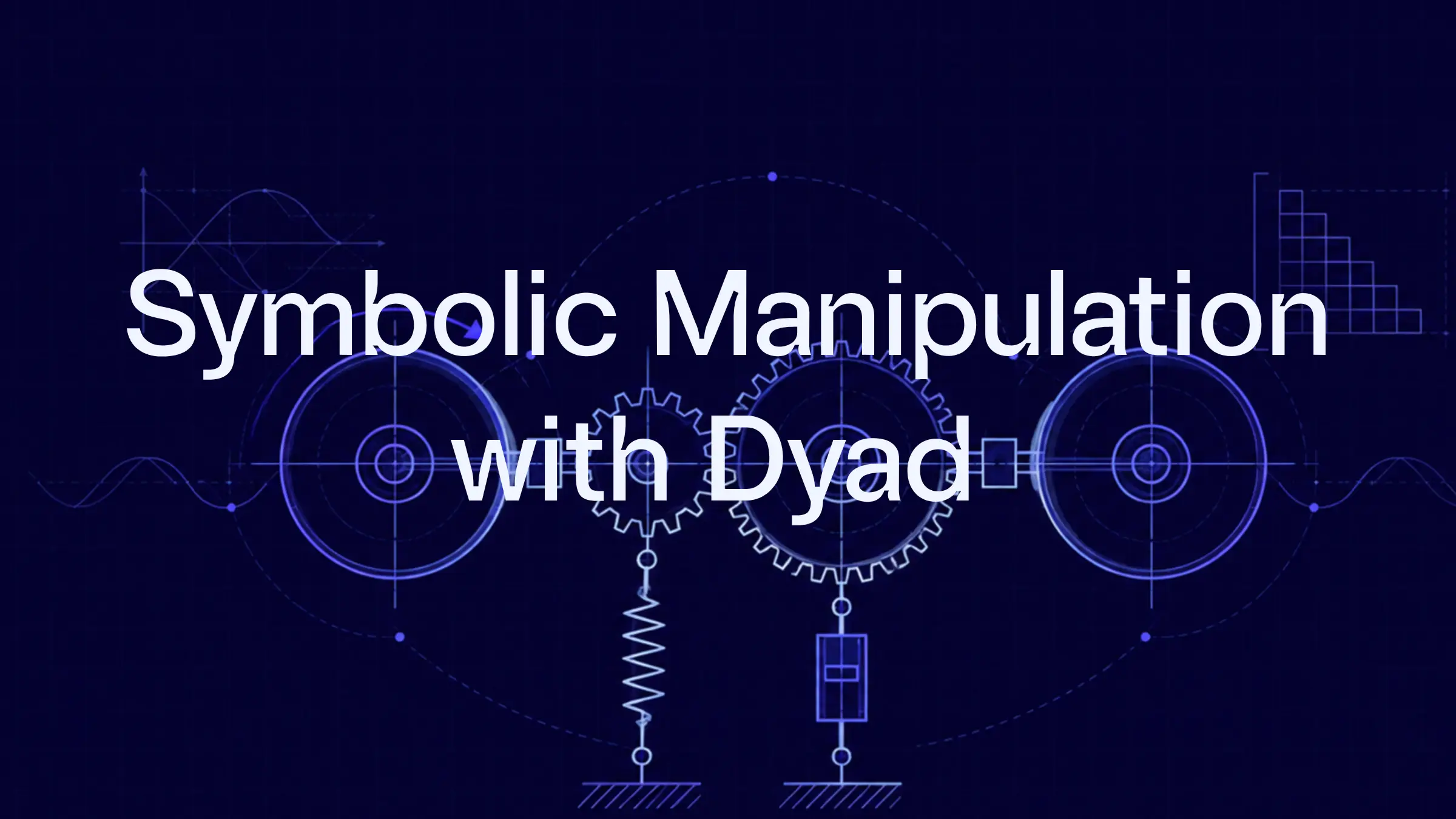

Engineers naturally think in components and connections. A rotating system might begin as a sketch: an inertia connected to a gear, another inertia, a spring, a damper, and an applied torque. The mathematics behind that sketch, however, can quickly become a large and tightly coupled system of equations.
In the third installment of our webinar series, we explored how symbolic manipulation bridges that gap in Dyad. The example we used follows a rotational mechanical model from an intuitive physical diagram to an efficient simulation, showing how the Dyad toolchain preserves the engineer’s original intent while automatically reorganizing the underlying mathematics for speed and reliability.
The central idea is simple: engineers should be able to focus on the physics of a system, while the modeling environment handles the tedious and error-prone work required to solve it.
Modeling systems the way engineers think
Dyad supports both graphical and textual representations of physical models. In the webinar example, the system included three rotational inertias, a gear, a spring, a damper connected to ground, and an external torque driven by a step input.
Each component contributes its own physical behavior. An inertia expresses conservation of angular momentum. A spring contributes Hooke’s law. A gear imposes kinematic and torque relationships. When these components are connected, they combine to form a complete mathematical description of the system.
This component-based approach closely resembles the way an engineer might draw a system on paper. But a connection line is more than a visual link: it has precise mathematical meaning.
For the rotational connectors used in the example, a connection does two things:
It sets the potential variables such as angular position equal at the connection point.
It requires the associated flow variables, such as torque to sum to zero.
Together, these relationships enforce the relevant conservation laws. In this case, they preserve angular momentum and, through the relationship between angular position and velocity, conserve energy as well.
The result is that a compact engineering diagram expands into a fully specified system of equations without requiring the modeler to derive every relationship by hand.
Why physical models lead to differential-algebraic equations
If the example contained only independent inertias, its equations would be straightforward ordinary differential equations, or ODEs. Adding springs and dampers would introduce forces and torques that could still be written explicitly in terms of the system’s positions and velocities.
An ideal gear changes the structure of the problem. A gear imposes algebraic constraints between the angles and angular velocities of two connected inertias. Those quantities can no longer vary independently. The model therefore becomes a system of differential-algebraic equations, or DAEs, combining dynamic equations with algebraic constraints.
This is not a modeling defect. DAEs arise naturally from meaningful physical systems, especially when components introduce rigid constraints. Restricting users to models that produce only explicit ODEs would rule out many useful and intuitive formulations.
Dyad instead embraces DAEs and uses the structure of the equations to transform them into forms that numerical solvers can handle efficiently.
The symbolic pipeline: making the equations smaller and easier to solve
The fully expanded system can contain many more equations than are ultimately necessary. Symbolic manipulation identifies redundancies, dependencies, and structural patterns before numerical integration begins.
The webinar highlighted four important techniques.
1. Alias elimination
Connections often create variables that are equal or differ only by a simple sign or scale factor. Alias elimination substitutes these relationships directly and removes redundant variables and equations.
In the demonstration, this first step reduced a system of roughly 30 equations to a much smaller one. Because the cost of solving a dense linear system can grow cubically with its size, even a seemingly modest reduction can produce a major performance improvement.
2. Equation sorting and block lower triangular form
The next step examines which unknowns appear in which equations. By reordering equations and variables, the compiler can often transform the system’s Jacobian into a lower triangular or block lower triangular (BLT) structure.

A lower triangular system can be solved efficiently through substitution rather than as one large simultaneous problem. A BLT system offers a similar advantage: most variables can be solved in sequence, while only the smaller coupled blocks require simultaneous solution.
This structural reordering can reduce work dramatically—from the cost of solving one large dense system to a sequence of much cheaper operations.
3. Index reduction
DAEs are commonly classified by their structural index. ODEs can be viewed as index-zero DAEs, while index-one systems are also well supported by established numerical methods. Higher-index DAEs are more difficult to solve directly.
The gear constraint in the webinar example produced a higher-index system and a singular Jacobian. Index reduction resolves this by differentiating selected constraint equations and incorporating the resulting relationships into the system. This exposes information about the derivatives of constrained variables and produces a lower-index problem with an invertible Jacobian.
The transformed equations remain consistent with the original physical model; they are simply expressed in a form that a numerical solver can use.
4. Tearing
Even after equation sorting and index reduction, a BLT system may contain coupled blocks. Tearing can reduce the size of those blocks by selecting one or more iteration variables and temporarily treating them as known.
The remaining variables can then be calculated through substitution. A smaller nonlinear iteration is used to update the selected tearing variables until the entire system is consistent.
In a small teaching example, this may only replace a four-by-four solve with a scalar iteration. In a production model, however, it can reduce a block containing hundreds of variables to one containing only a few.
Symbolic knowledge unlocks further optimization
The value of a symbolic representation goes beyond recognizing zeros in a matrix. Because the toolchain can inspect the equations themselves, it can determine whether a system is linear, nonlinear, time-varying, or time-invariant.
Those distinctions matter. Newton–Raphson iteration, for example, converges in a single step for a linear system. If a matrix is also time-invariant, it can be factored or inverted once at the beginning of a simulation and reused at every time step.
By contrast, a purely numerical tool that only samples inputs and residuals sees isolated evaluations rather than the complete structure of the problem. It may have to approximate the Jacobian through finite differences and rediscover sparsity repeatedly. A symbolic system begins with a global view and can plan the computation before the simulation starts.
Preserving consistency through state selection and initialization
Index reduction introduces another important consideration: not every differentiated variable is an independent state.
In the geared system, the two connected angles are related, as are the two angular velocities. Although four differentiated variables appear in the equations, only two independent state variables are required. The system must therefore select a valid combination of states and calculate consistent initial values for the remaining variables.
This process is known as state selection. It ensures that the simulation begins on the constraint manifold defined by the original equations.
Numerical integration can also introduce small errors that cause algebraic constraints to drift over time. The Dyad toolchain uses techniques such as dummy derivatives to control this drift. Dynamic state selection can also change the chosen states during simulation if the current selection leads to a singular Jacobian.
These details are crucial: optimization is valuable only if the transformed problem continues to represent the model the engineer intended.
Automation lets engineers focus on physics
It is possible to perform alias elimination, equation sorting, index reduction, state selection, and tearing by hand for a small example. At a realistic scale, it becomes impractical. A model with tens of thousands of equations would make manual restructuring slow, difficult to maintain, and highly susceptible to errors.
The Dyad toolchain automates this work using deterministic, well-established algorithms. Many of the underlying symbolic capabilities are provided by ModelingToolkit.jl, a cornerstone of the broader Dyad product, alongside the Dyad language and agent, Julia, and the surrounding development environment.
This combination gives engineers the freedom to construct systems from reusable physical components, explore model variations, and iterate quickly—without repeatedly translating their work into solver-friendly block diagrams or manually optimized equations.
The key takeaway
Symbolic manipulation is what allows an intuitive physical model to become an efficient numerical simulation.
Starting from components and connections, the Dyad toolchain generates the governing equations, removes redundant aliases, reveals the system’s block structure, reduces the DAE index, selects consistent states, and tears large coupled systems into smaller problems. Throughout those transformations, it preserves consistency with the equations defined by the modeler.
The payoff is not only faster simulation. It is a better engineering workflow: model the physics in a natural form, let the compiler handle the mathematical bookkeeping, and spend more time designing and understanding the system itself.
Watch the full webinar here.