The implementation of a control system often starts in a simulation environment. Having successfully tested that the system works as intended in simulation, the job of deploying it to the target hardware begins. Not seldom, this deployment step entails a rewrite of the controller in a language for which there exists a compiler for the target platform, often the C programming language. Since the control system already exists in one form, the implementation in the simulation model, we should in principle have most of the information required to perform this rewrite and deployment automatically! In a recent webinar we walked through this path with the Dyad modeling language for a rotary pendulum. We constructed a multibody model of the physical device, a discrete-time swing-up controller closed around that model, and then the same controller, automatically exported as C code. We showed how the generated code could be automatically copied to a Raspberry Pi, compiled and executed against the physical pendulum. This post summarizes what was shown and what made it work. The recording is embedded below and the models are available in the QuanserComponents.jl repository.

The system

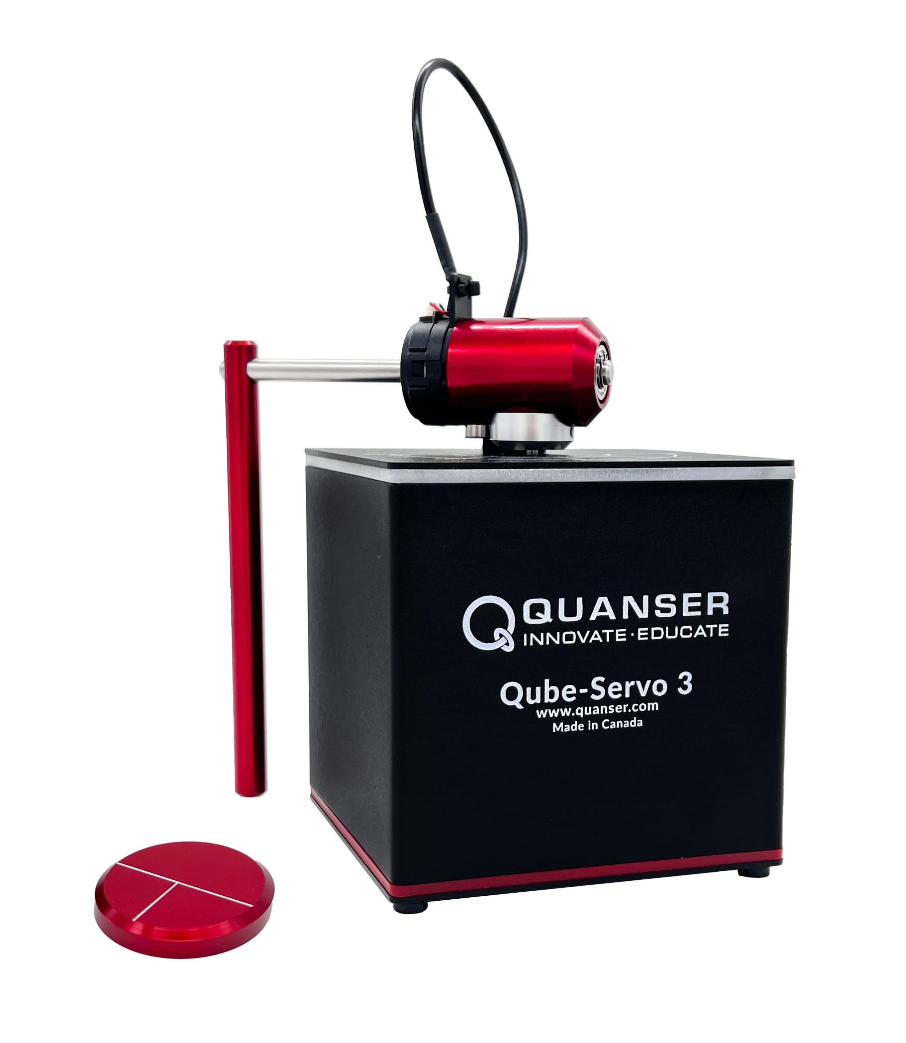
The device is a Quanser QUBE-Servo with the rotary pendulum attachment, a configuration known as a Furuta pendulum. A DC motor in the base drives a horizontal arm, and a pendulum rod hangs from a free hinge at the end of the arm. We refer to the actuated joint as the shoulder and the free joint as the elbow. Both angles are measured by encoders, and the motor voltage is the only control input. The control objective is to make the pendulum swing up from its initial condition of hanging down, and then stabilize it in the upright position, a common project in university control classes.

The multibody plant model

To design and verify the controller before interfacing the hardware, we need a simulation model. This model was built with the Dyad multibody standard library: a fixed base, a revolute joint for the shoulder driven by a DC-motor component and a friction component, a body for the upper arm, a second revolute joint for the elbow with a viscous damper, and a body for the pendulum rod. Angle sensors on the two joints provide the two measured outputs. The mass, length and inertia parameters were identified from experiments on the device (see video series for more details on these experiments).

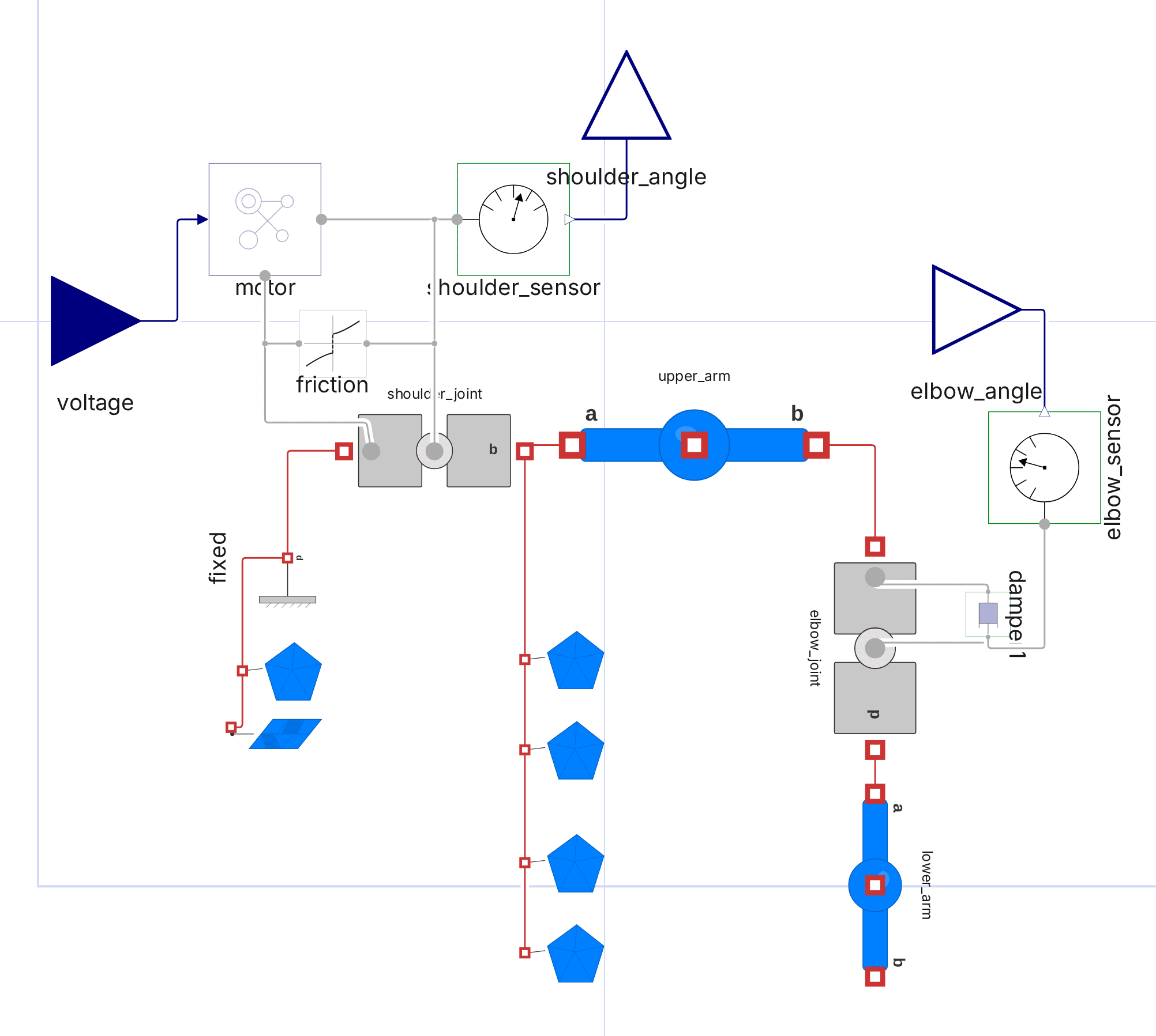
Apart from the dynamic components, the blue components along the bottom of the diagram add CAD geometry to the device for animation purposes:

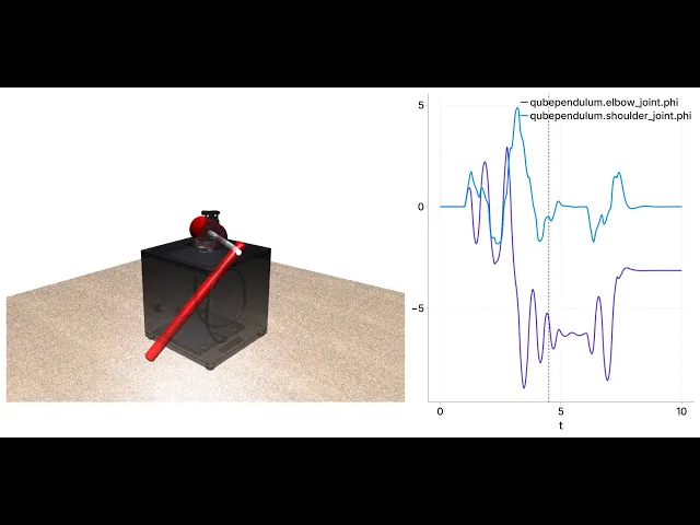
The animation is rendered directly from the simulation result. The pendulum angle (purple) settles at $-\pi$ (upright), after a second swing-up attempt. To exercise recovery and homing logic in the controller, the simulation scenario includes plant parameter mismatch where the controller was tuned for the datasheet parameters while the plant uses parameters identified from data, causing the initial attempt to fail.

The controller as a synchronous program

The closed loop system is a hybrid model. The plant is a continuous-time system, while the controller is a discrete-time system that executes once every 5 ms. In Dyad, the transition between the two is explicitly modeled: sampler components take measurements of the angles, a zero-order hold component acting on the control signal interpolates it from discrete to continuous time, and a clock component that assigns the clock to the synchronous program. Dashed connections indicate clocked signals and solid connections indicate continuous ones.

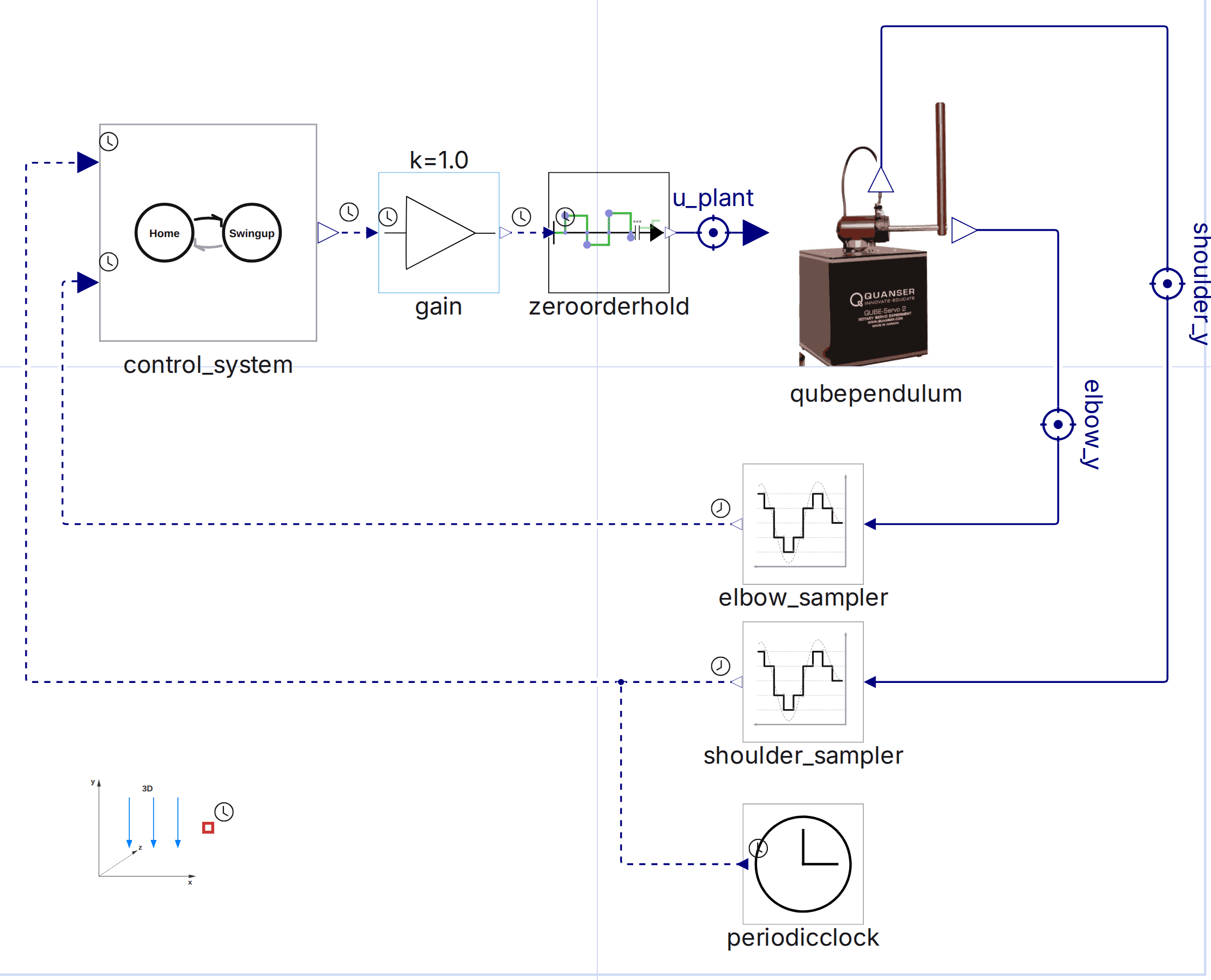
The controller has two main modes of operation:

• Energy-based swing-up. The energy of the pendulum, $E = \tfrac{1}{2} J \dot\alpha^2 + m g l (1 + \cos\alpha)$, where $\alpha$ is the pendulum angle measured from upright, is compared to the energy of the upright rest position, $E_\text{ref} = 2 m g l$. The motor voltage $u = k_E (E - E_\text{ref}) \, \operatorname{sign}(\dot\alpha \cos\alpha) - k_\theta \theta$ pumps energy into the pendulum in the correct phase, while the term on the arm angle $\theta$ keeps the arm near its center. The voltage is saturated at $\pm 3$ V to keep the hardware from tearing itself apart if something goes wrong.

• LQR stabilization. Once the pendulum is within a small angle of upright, a linear state-feedback controller takes over. Its gain was computed by linearizing the same multibody model about the upright equilibrium, discretizing it at the sample interval of the clock and solving a discrete-time LQR problem. Dyad includes features for all of these steps to be handled automatically. The velocities are not measured; they are estimated by differentiating the encoder angles and low-pass filtering the result. The diagram of the control system is shown below.

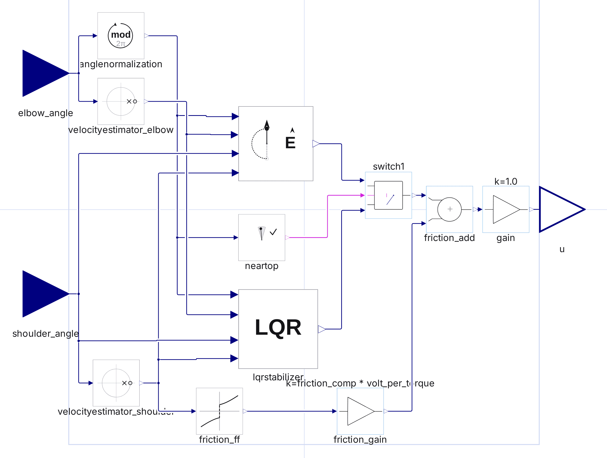
Around this core sit two supervisory functions: a homing controller that centers the arm before a swing-up attempt, and an error-recovery mode that re-homes the arm if it stays outside its allowed range for too long. Together they form a small state machine built from unit delays and switches. Dyad does not yet have dedicated state-machine support, which is an upcoming feature.

The same controller on the hardware

To run on the device, the same control system is instead connected to a model of the hardware device: one component reads the encoders, measurement and one writes the motor voltage, command. A diagnostics component records the achieved sample period and the execution time of each tick, and a data logger writes data to a file. The controller in the middle is the same component as in the simulation model.

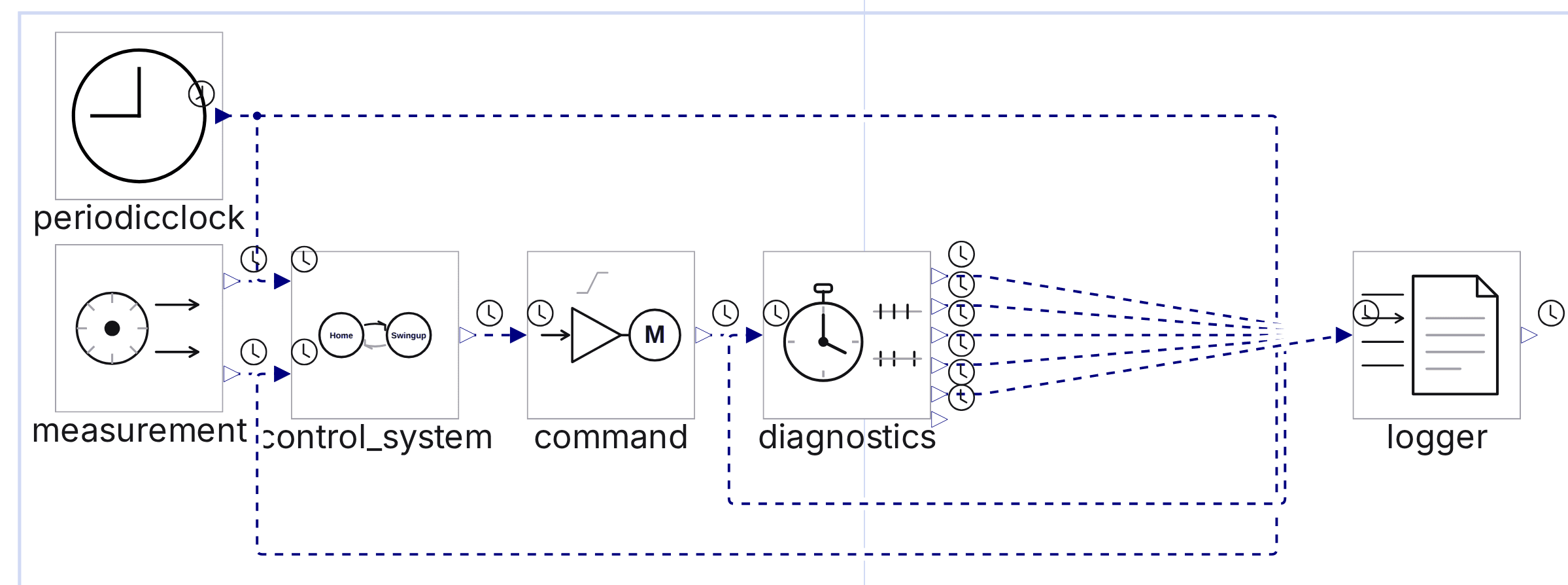
We can look into one of the hardware-communication components to understand how they are implemented. The command component consists of declarations and a single equation:

component HardwareCommand@[input clk extends Discrete]
  u = Dyad.RealInput@[clk]()
  u_applied = Dyad.RealOutput@[clk]()
  parameter umax::Dyad.Voltage = 10.0
relations
  u_applied@clk = hw_write(u, umax)
end

component HardwareCommand@[input clk extends Discrete]
  u = Dyad.RealInput@[clk]()
  u_applied = Dyad.RealOutput@[clk]()
  parameter umax::Dyad.Voltage = 10.0
relations
  u_applied@clk = hw_write(u, umax)
end

component HardwareCommand@[input clk extends Discrete]
  u = Dyad.RealInput@[clk]()
  u_applied = Dyad.RealOutput@[clk]()
  parameter umax::Dyad.Voltage = 10.0
relations
  u_applied@clk = hw_write(u, umax)
end

The equation calls hw_write, a Julia function. Dyad models can directly call Julia functions, and this particular Julia function performs a call into a small C library that wraps the hardware vendor's interface:

hw_write(u::Real, umax::Real)::Float64 =
    ccall((:qube_hw_write, QUBE_HW_LIB), Cdouble, (Cdouble, Cdouble), u, umax

hw_write(u::Real, umax::Real)::Float64 =
    ccall((:qube_hw_write, QUBE_HW_LIB), Cdouble, (Cdouble, Cdouble), u, umax

hw_write(u::Real, umax::Real)::Float64 =
    ccall((:qube_hw_write, QUBE_HW_LIB), Cdouble, (Cdouble, Cdouble), u, umax

When the program runs in Julia, the ccall invokes the shared library directly, and when the program is exported as C, the code generator recognizes the ccall and emits an extern declaration and a call to the same C function, so the generated program links against the same library with no Julia involved.

Compile, deploy and run from the play button

Compiling the program, exporting C, copying it to the Raspberry Pi, building and running it there and streaming the log back is a sequence of steps that nobody wants to repeat by hand. In Dyad, such a sequence is packaged as an analysis: a Dyad definition with parameters, implemented in Julia behind the scenes. Such an analysis may be executed by pressing the play button in the graphical editor or by calling it from Julia.

analysis FurutaSwingupExperiment
  extends FurutaSwingupBase(run = true, live_plot = true, deploy_host = "user@192.168.1.49")
  model = FurutaHardware()
relations
end

analysis FurutaSwingupExperiment
  extends FurutaSwingupBase(run = true, live_plot = true, deploy_host = "user@192.168.1.49")
  model = FurutaHardware()
relations
end

analysis FurutaSwingupExperiment
  extends FurutaSwingupBase(run = true, live_plot = true, deploy_host = "user@192.168.1.49")
  model = FurutaHardware()
relations
end

The parameters of the this particular analysis include the sample interval, the LQR weights, the duration of the run, whether to export C, and the host to deploy to. Running the analysis in the webinar took a few seconds: the program was compiled, the sources were copied, make was invoked on the Raspberry Pi, the program was started, and a live plot of the log appeared while the pendulum swung up. Anyone can author an analysis, in the same way that anyone can author a component model.

The generated C is long, roughly ten thousand lines for this controller, but it is traceable. Each generated statement is associated with a comment indicating the Dyad equation it stems from, and each generated function indicates the Julia function it was generated from. In regulated fields, this provenance from model to code is required before generated code may be used in production.

Why C, and what was left out

The Raspberry Pi is capable of running Julia, and the same analysis can run the program on the Julia backend instead. C export exists for the targets that cannot run Julia, which are typically smaller, as well as for workflows that require C.

The video series on the pendulum covers a few extra topics, the actual design of the control system as well as parameter and friction identification. The models, the C library and the analyses are open in the QuanserComponents.jl repository, which also includes Dyad programs to perform friction and parameter estimation. Finally, the Dyad documentation is available at help.juliahub.com/dyad.

Conclusion

When a control system is working in simulation, the implementation effort would ideally be over. Dyad now supports code generation which brings this dream closer to reality. We have demonstrated how Dyad supports the entire workflow from plant modeling and control system design, to deployment and execution. The models used during the webinar and referenced in this post are openly available, please try these features out today!